Prosocial Regulatory Focus

Study 2 Examining Seven Mindsets

Authors
Affiliations

Zihan Hei

Binghamton University

Shane McCarty

Binghamton University

Promote Care & Prevent Harm

Jordan Booker

University of Missouri

Kyle Pacque

Promote Care & Prevent Harm

Heather Orom

University at Buffalo

Published

April 15, 2025

Abstract

Promotion motivation and prevention motivation are two distinct motivational orientations, rooted in the promotion and prevention motivation systems, that influence whether one focuses on approaching gains and avoiding non-gains as well as approaching non-losses and avoiding losses, respectively. Individuals with a chronic preference for promotion focus are more likely to select promotion goals (that produce gains) and eager strategies; whereas people with a dominant prevention focus are more likely to select prevention goals (that produce non-losses) and vigilant strategies. More than two decades of reseach on regulatory focus theory shows motivational orientation influences health behavior, work behavior, and prosocial behavior (Scholer et al., 2019). However, promotion/prevention motivation has not been integrated with prosocial motivation to explain the goal pursuit strategy for prosocial behavior that benefits the health, safety, and wellbeing of others. In this pilot study, we examine the seven mindset types of prosocial regulatory focus: promote care, prevent harm, fail to care, fail to harm, maintain care, respond to harm, and flipping from harm to care.

Keywords

prosocial regulatory focus, pilot study

Show the code
library(rmarkdown)
library(readr)

df <- read_csv("02.13.24.Mindsets.Data.csv")
Rows: 121 Columns: 67
── Column specification ────────────────────────────────────────────────────────
Delimiter: ","
chr  (10): test, demo1, demo2, demo3, demo4, demo5, demo6, demo7, trainingda...
dbl  (56): participantID, consent, PROMOTECARE, PREVENTHARM, FAILCARE, FAILH...
time  (1): time

ℹ Use `spec()` to retrieve the full column specification for this data.
ℹ Specify the column types or set `show_col_types = FALSE` to quiet this message.
Show the code
head(df)
# A tibble: 6 × 67
  participantID time   consent test    PROMOTECARE PREVENTHARM FAILCARE FAILHARM
          <dbl> <time>   <dbl> <chr>         <dbl>       <dbl>    <dbl>    <dbl>
1        123456 53:09        1 5               7.8         7        4.4      4.8
2        789101 42:05        1 5               8.4         3.8      4.8      3.8
3        121314 00:09        1 5               7.8         6.4      7        6.6
4        151617 24:12        1 Not at…         6           2.2      5.6      3.8
5        506137 09:31        1 5               8.6         5        3.4      4.6
6        379463 43:34        1 Not at…         7.8         5        4.8      5  
# ℹ 59 more variables: MAINTAIN <dbl>, FLIP <dbl>, RESPOND <dbl>,
#   promotecare1 <dbl>, preventharm1 <dbl>, failcare1 <dbl>,
#   preventharm2 <dbl>, promotecare2 <dbl>, preventharm3 <dbl>,
#   promotecare3 <dbl>, failharm1 <dbl>, failcare2 <dbl>, failharm2 <dbl>,
#   promotecare4 <dbl>, preventharm4 <dbl>, failcare3 <dbl>, failharm3 <dbl>,
#   failcare4 <dbl>, failharm4 <dbl>, promotecare5 <dbl>, failharm5 <dbl>,
#   failcare5 <dbl>, preventharm5 <dbl>, maintain1 <dbl>, flip1 <dbl>, …
Show the code
library(ggplot2)
library(ggplot2)
library(plotly)

Attaching package: 'plotly'
The following object is masked from 'package:ggplot2':

    last_plot
The following object is masked from 'package:stats':

    filter
The following object is masked from 'package:graphics':

    layout
Show the code
library(dplyr)

Attaching package: 'dplyr'
The following objects are masked from 'package:stats':

    filter, lag
The following objects are masked from 'package:base':

    intersect, setdiff, setequal, union
Show the code
library(tidyr)
library(ggrain)
Registered S3 methods overwritten by 'ggpp':
  method                  from   
  heightDetails.titleGrob ggplot2
  widthDetails.titleGrob  ggplot2

1 Descriptives

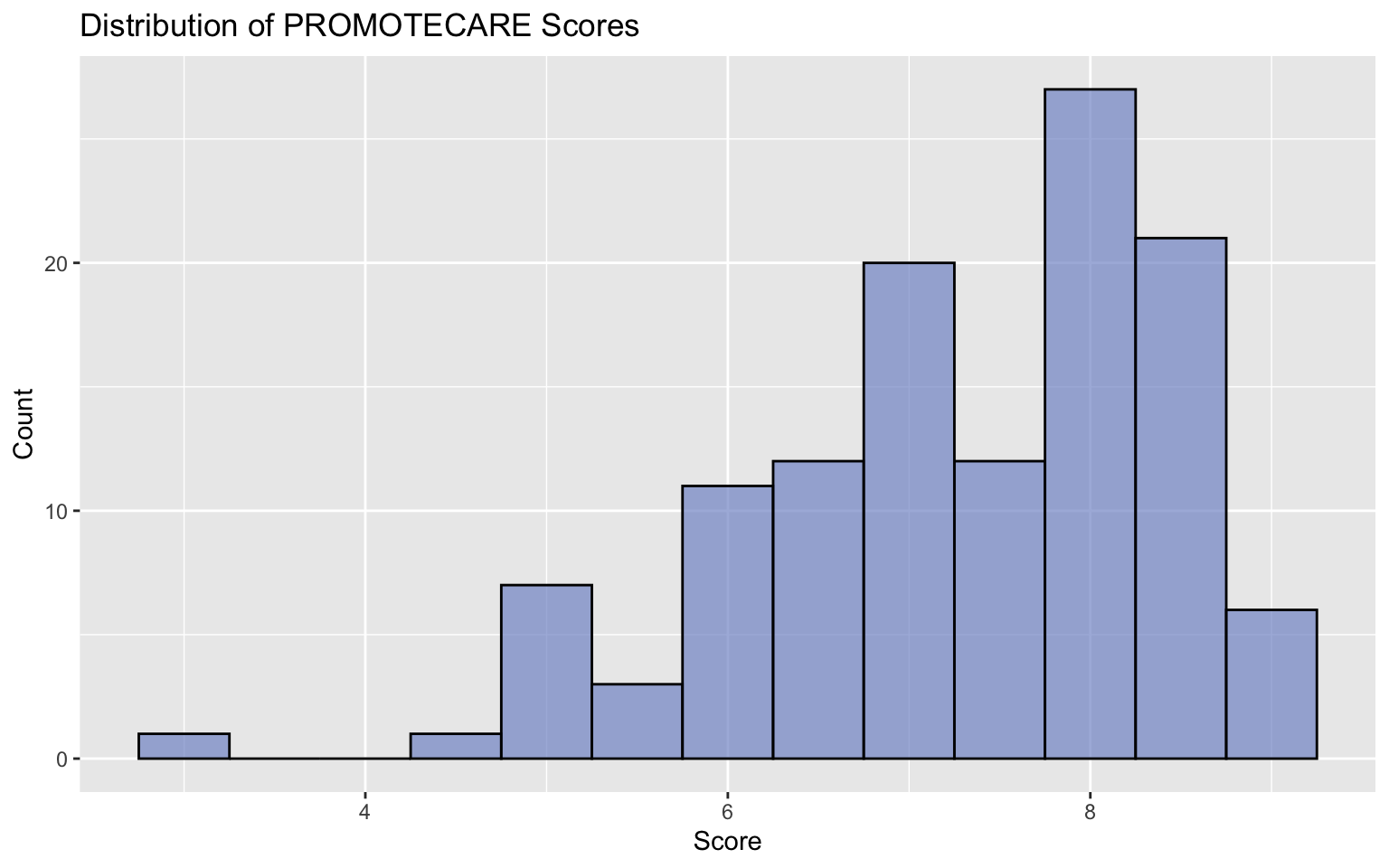
1.1 Distribution of Promoting Care Mindset

Show the code
## Distribution of PROMOTECARE
distri_of_procare <- ggplot(df, aes(x=PROMOTECARE)) + 
  geom_histogram(binwidth=0.5, fill="#8297ce", color = "black", alpha=0.7) +
  labs(title="Distribution of PROMOTECARE Scores", x="Score", y="Count")

distri_of_procare

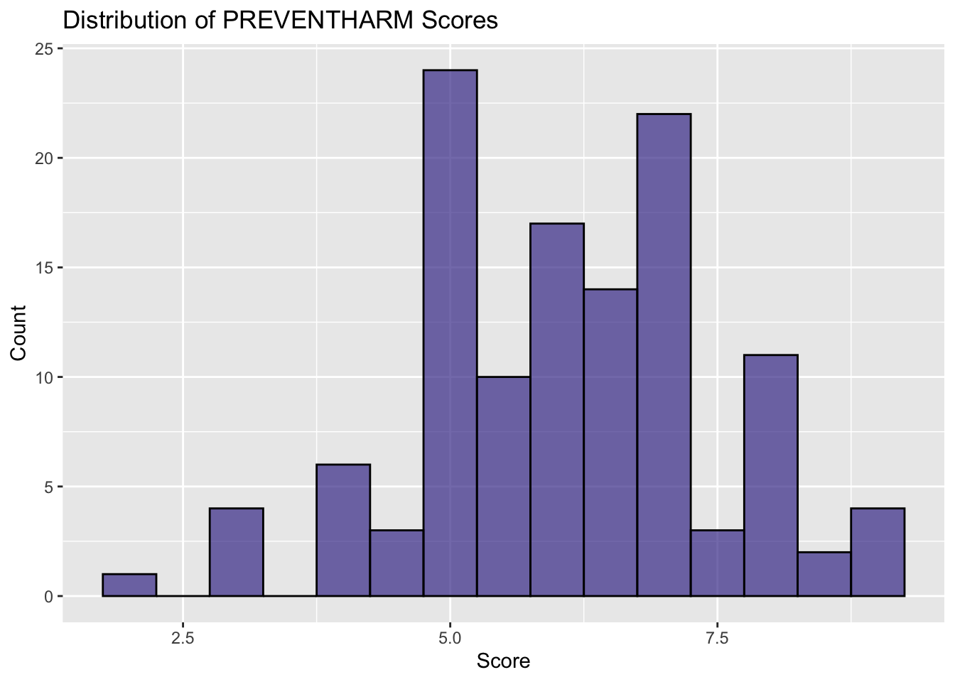
1.2 Distribution of Preventing Harm Mindset

Show the code
distri_of_preharm <- ggplot(df, aes(x=PREVENTHARM)) + 
  geom_histogram(binwidth=0.5, fill="#453a98", color = "black", alpha=0.7) +
  labs(title="Distribution of PREVENTHARM Scores", x="Score", y="Count")

distri_of_preharm

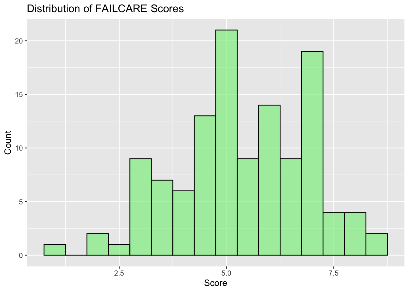
1.3 Distribution of Failing to Care Mindset

Show the code
## Distribution of FAILCARE
#| echo: true

distri_of_failcare <- ggplot(df, aes(x=FAILCARE)) + 
  geom_histogram(binwidth=0.5, fill="#90EE90", color = "black", alpha=0.7) +
  labs(title="Distribution of FAILCARE Scores", x="Score", y="Count")

distri_of_failcare

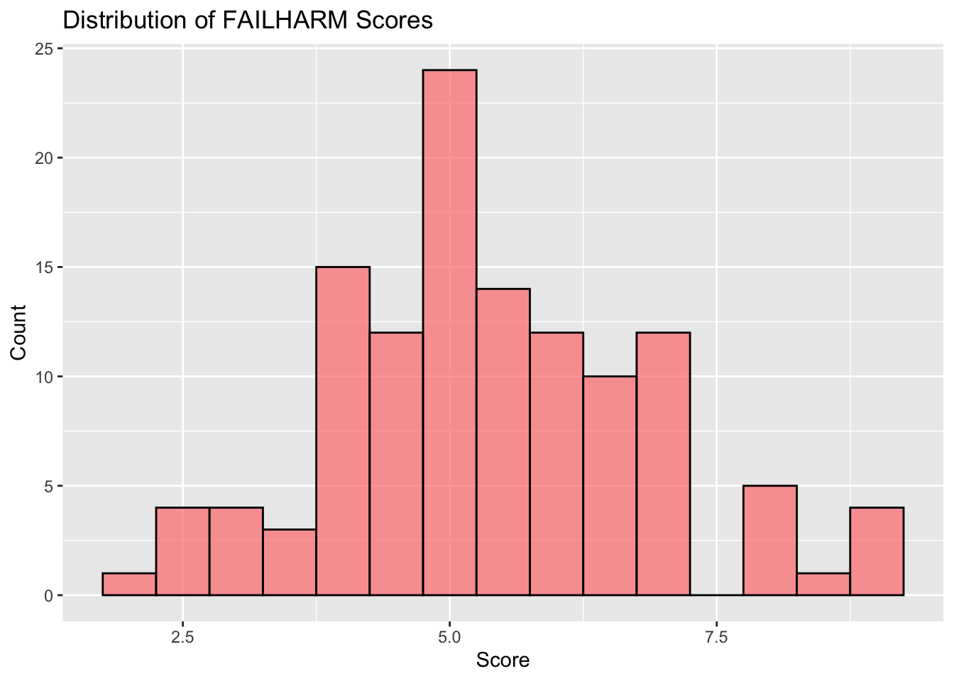
1.4 Distribution of Failing to Prevent Harm Mindset

Show the code
## Distribution of FAILHARM

distri_of_failharm <- ggplot(df, aes(x=FAILHARM)) + 
  geom_histogram(binwidth=0.5, fill="#FF7F7F", color = "black", alpha=0.7) +
  labs(title="Distribution of FAILHARM Scores", x="Score", y="Count")

distri_of_failharm

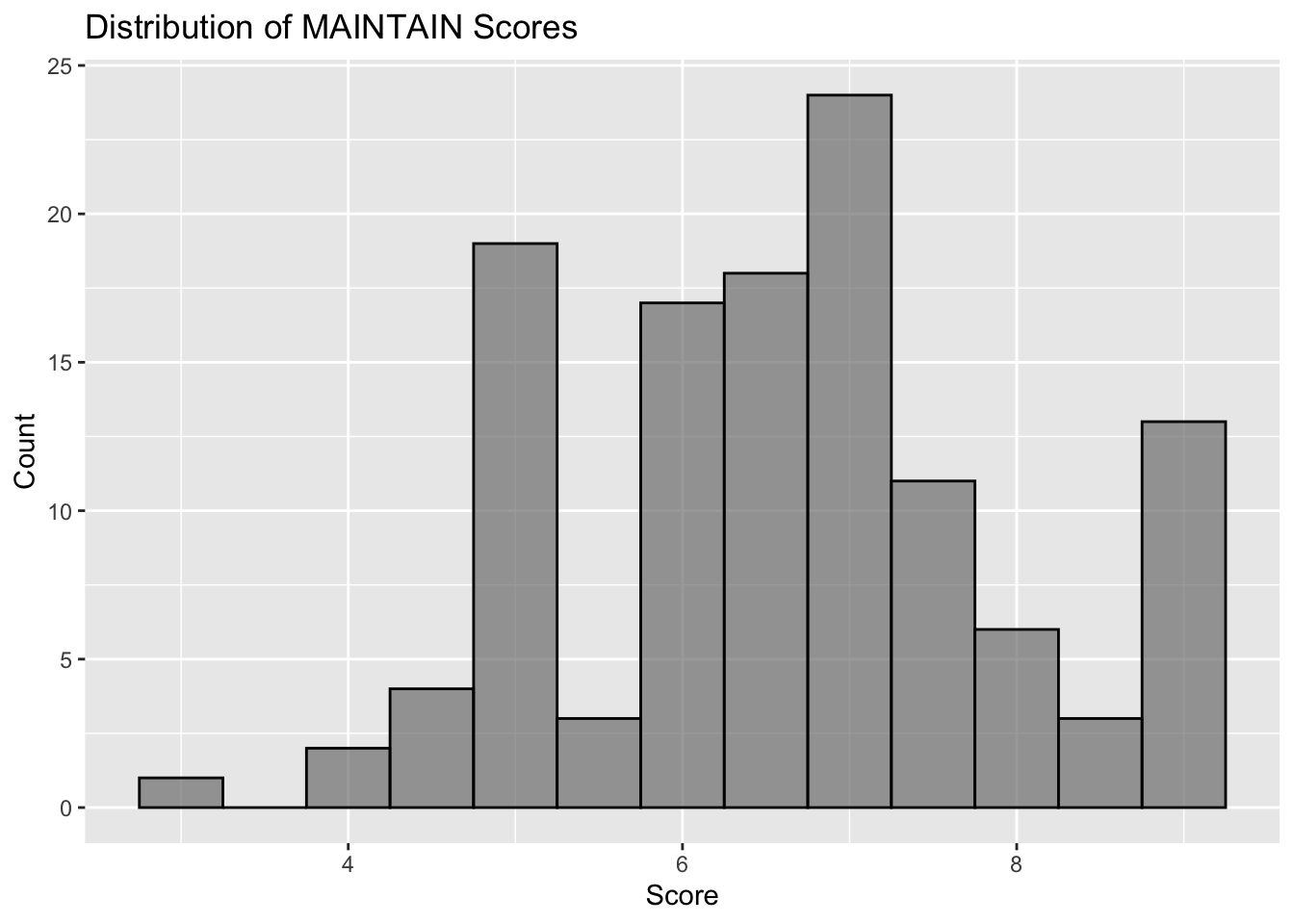
1.5 Distribution of Maintaining Care Mindset

Show the code
## Distribution of MAINTAIN

distri_of_maintain <- ggplot(df, aes(x=MAINTAIN)) + 
  geom_histogram(binwidth=0.5, fill="#808080", color = "black", alpha=0.7) +
  labs(title="Distribution of MAINTAIN Scores", x="Score", y="Count")

distri_of_maintain

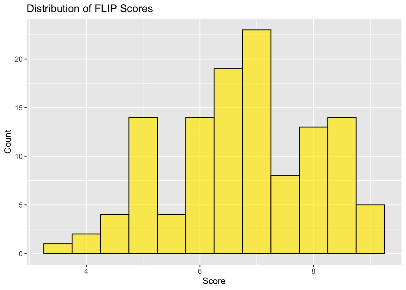
1.6 Distribution of Flipping from Harm to Care Mindset

Show the code
## Distribution of FLIP

distri_of_flip <- ggplot(df, aes(x=FLIP)) + 
  geom_histogram(binwidth=0.5, fill="#FFEA00", color = "black", alpha=0.7) +
  labs(title="Distribution of FLIP Scores", x="Score", y="Count")

distri_of_flip

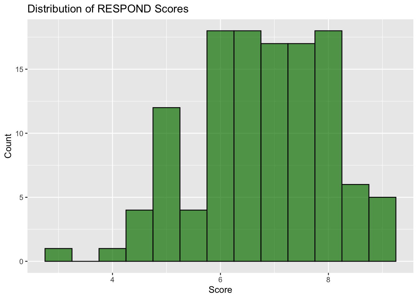
1.7 Distribution of Responding to Harm

Show the code
## Distribution of RESPOND

distri_of_respond <- ggplot(df, aes(x=RESPOND)) + 
  geom_histogram(binwidth=0.5, fill="#008000", color = "black", alpha=0.7) +
  labs(title="Distribution of RESPOND Scores", x="Score", y="Count")

distri_of_respond

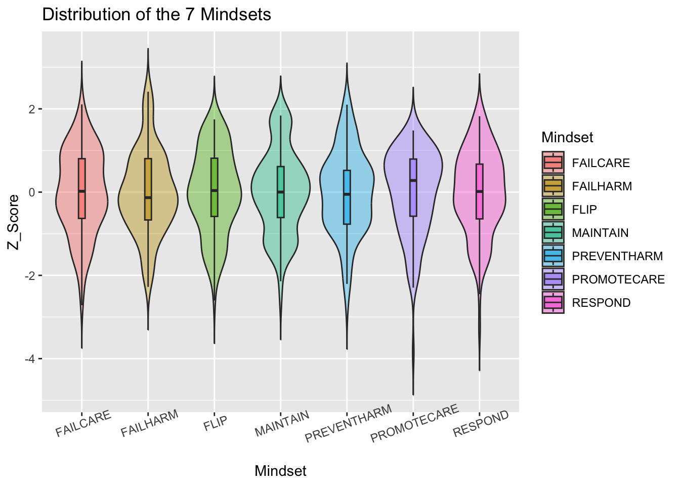
1.8 Distribution of Seven Mindsets

Show the code
mindsets <- c("PROMOTECARE", "PREVENTHARM", "FAILCARE", "FAILHARM", "MAINTAIN", "FLIP", "RESPOND")

## standardize all mindset variables to z-scores
df_z <- df %>%
  mutate(across(all_of(mindsets), ~ as.numeric(scale(.x))))


## reshape to long format
df_long <- df_z %>%
  select(all_of(mindsets)) %>%
  pivot_longer(cols = everything(), names_to = "Mindset", values_to = "Z_Score")

df_long
# A tibble: 847 × 2
   Mindset     Z_Score
   <chr>         <dbl>
 1 PROMOTECARE   0.451
 2 PREVENTHARM   0.666
 3 FAILCARE     -0.632
 4 FAILHARM     -0.401
 5 MAINTAIN     -0.152
 6 FLIP         -0.429
 7 RESPOND       0.508
 8 PROMOTECARE   0.966
 9 PREVENTHARM  -1.63 
10 FAILCARE     -0.371
# ℹ 837 more rows
Show the code
## Distribution of the 7 mindsets

distr_allmindset <- ggplot(df_long, aes(x = Mindset, y = Z_Score, fill = Mindset)) +
  geom_violin(trim = FALSE, alpha = 0.4) +
  geom_boxplot(width = 0.1, outlier.shape = NA, alpha = 0.6) +
  labs(title = "Distribution of the 7 Mindsets",
       y = "Z_Score", x = "Mindset") +
  theme(axis.text.x = element_text(angle = 20))


distr_allmindset

2 Mindset Associations

The correlation heatmap shows the correlations among the seven mindsets with green-yellow indicating the strongest, positive correlations.

  • FAILHARM & FAILCARE: Since both mindsets represent anxiety about not meeting one’s caregiving goals, it makes sense that they are positively correlated (r = 0.66).

  • PROMOTECARE & MAINTAIN: A strong correlation (r = 0.67) suggests that individuals who emphasize promote care also tend to maintain it.This makes sense because those who focus on creating positive outcomes (PROMOTECARE) are also likely to be committed to sustaining those outcomes (MAINTAIN).

(expand.grid(): creates all combinations of the column names (X) and row names (Y) of the matrix. https://www.statology.org/expand-grid-r/)

Show the code
## Heatmap of all mindsets relationships

## filter out all the mindsets
allmindsets <- df %>% select(PROMOTECARE, PREVENTHARM, FAILCARE, FAILHARM, MAINTAIN, FLIP, RESPOND)

## computes the correlation matrix between all selected variables ("complete.obs" make sure we only use non-missing data)
corr_matrix <- cor(allmindsets, use="complete.obs")

corr_matrix
            PROMOTECARE PREVENTHARM   FAILCARE  FAILHARM  MAINTAIN       FLIP
PROMOTECARE   1.0000000   0.4209721 0.18803824 0.2208094 0.6688560 0.53918122
PREVENTHARM   0.4209721   1.0000000 0.16005895 0.4318124 0.3883044 0.60430001
FAILCARE      0.1880382   0.1600589 1.00000000 0.6577583 0.3186145 0.03352214
FAILHARM      0.2208094   0.4318124 0.65775827 1.0000000 0.3235537 0.22362933
MAINTAIN      0.6688560   0.3883044 0.31861454 0.3235537 1.0000000 0.53933114
FLIP          0.5391812   0.6043000 0.03352214 0.2236293 0.5393311 1.00000000
RESPOND       0.5801855   0.5527159 0.20594128 0.4130674 0.6350966 0.55208928
              RESPOND
PROMOTECARE 0.5801855
PREVENTHARM 0.5527159
FAILCARE    0.2059413
FAILHARM    0.4130674
MAINTAIN    0.6350966
FLIP        0.5520893
RESPOND     1.0000000
Show the code
## creates all combinations of the column names (X) and row names (Y) of the matrix
heatmap_data <- expand.grid(X = colnames(corr_matrix), Y = rownames(corr_matrix))

## convert correlation matrix into long vector, add a new column z contain the corr_matrix for each (x, y) pair
heatmap_data$Z <- as.vector(corr_matrix)

heatmap_data
             X           Y          Z
1  PROMOTECARE PROMOTECARE 1.00000000
2  PREVENTHARM PROMOTECARE 0.42097215
3     FAILCARE PROMOTECARE 0.18803824
4     FAILHARM PROMOTECARE 0.22080943
5     MAINTAIN PROMOTECARE 0.66885600
6         FLIP PROMOTECARE 0.53918122
7      RESPOND PROMOTECARE 0.58018553
8  PROMOTECARE PREVENTHARM 0.42097215
9  PREVENTHARM PREVENTHARM 1.00000000
10    FAILCARE PREVENTHARM 0.16005895
11    FAILHARM PREVENTHARM 0.43181238
12    MAINTAIN PREVENTHARM 0.38830441
13        FLIP PREVENTHARM 0.60430001
14     RESPOND PREVENTHARM 0.55271594
15 PROMOTECARE    FAILCARE 0.18803824
16 PREVENTHARM    FAILCARE 0.16005895
17    FAILCARE    FAILCARE 1.00000000
18    FAILHARM    FAILCARE 0.65775827
19    MAINTAIN    FAILCARE 0.31861454
20        FLIP    FAILCARE 0.03352214
21     RESPOND    FAILCARE 0.20594128
22 PROMOTECARE    FAILHARM 0.22080943
23 PREVENTHARM    FAILHARM 0.43181238
24    FAILCARE    FAILHARM 0.65775827
25    FAILHARM    FAILHARM 1.00000000
26    MAINTAIN    FAILHARM 0.32355367
27        FLIP    FAILHARM 0.22362933
28     RESPOND    FAILHARM 0.41306736
29 PROMOTECARE    MAINTAIN 0.66885600
30 PREVENTHARM    MAINTAIN 0.38830441
31    FAILCARE    MAINTAIN 0.31861454
32    FAILHARM    MAINTAIN 0.32355367
33    MAINTAIN    MAINTAIN 1.00000000
34        FLIP    MAINTAIN 0.53933114
35     RESPOND    MAINTAIN 0.63509656
36 PROMOTECARE        FLIP 0.53918122
37 PREVENTHARM        FLIP 0.60430001
38    FAILCARE        FLIP 0.03352214
39    FAILHARM        FLIP 0.22362933
40    MAINTAIN        FLIP 0.53933114
41        FLIP        FLIP 1.00000000
42     RESPOND        FLIP 0.55208928
43 PROMOTECARE     RESPOND 0.58018553
44 PREVENTHARM     RESPOND 0.55271594
45    FAILCARE     RESPOND 0.20594128
46    FAILHARM     RESPOND 0.41306736
47    MAINTAIN     RESPOND 0.63509656
48        FLIP     RESPOND 0.55208928
49     RESPOND     RESPOND 1.00000000
Show the code
## convert X and Y to factors with desired order
desired_order <- c("PROMOTECARE", "PREVENTHARM", "MAINTAIN", "RESPOND", "FLIP", "FAILCARE", "FAILHARM")
heatmap_data$X <- factor(heatmap_data$X, levels = desired_order)
heatmap_data$Y <- factor(heatmap_data$Y, levels = desired_order)
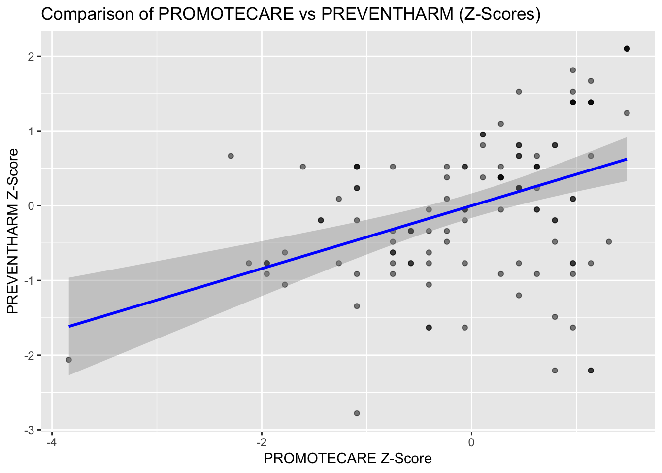
Show the code
mindsets_relation <- plot_ly(
  type = "heatmap",
  x = heatmap_data$X, 
  y = heatmap_data$Y, 
  z = heatmap_data$Z, 
  text = round(heatmap_data$Z, 2),
  texttemplate = "%{text}",
  hovertemplate = "<b>Correlation Details</b><br><b>X:</b> %{x}<br><b>Y:</b> %{y}<br><b>r:</b> %{z}<extra></extra>",
  colorbar = list(title = "Correlation Level (r): <br>")
  ) %>% 
  plotly::layout(
    title = "Mindset Correlation Heatmap",
    xaxis = list(title = ""),
    yaxis = list(title = "")
  )

mindsets_relation

2.1 Promoting Care & Preventing Harm Mindsets

Show the code
## Standardize variables to z-scores
df$PROMOTECARE_zscore <- as.numeric(scale(df$PROMOTECARE))
df$PREVENTHARM_zscore <- as.numeric(scale(df$PREVENTHARM))

## compare promotecare & preventharm by scatter plot
ggplot(df, aes(x = PROMOTECARE_zscore, y = PREVENTHARM_zscore)) +
  geom_point(alpha = 0.5) +                       
  geom_smooth(method = "lm", color = "blue") +   
  labs(title = "Comparison of PROMOTECARE vs PREVENTHARM (Z-Scores)",
       x = "PROMOTECARE Z-Score", y = "PREVENTHARM Z-Score")
`geom_smooth()` using formula = 'y ~ x'

3 Differences by Sociodemographics

3.1 Promoting Care Mindset by Gender Identity

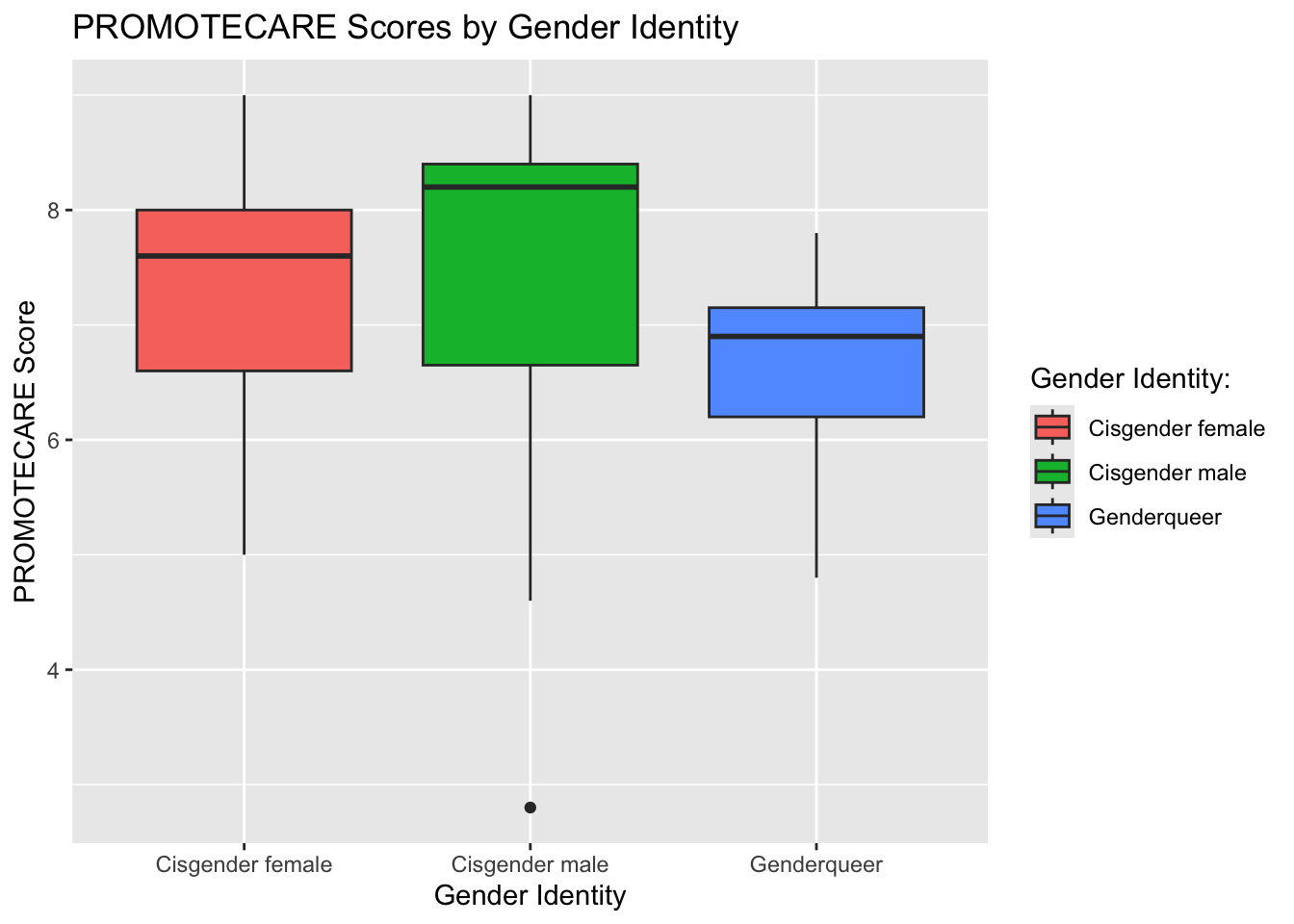
  • According to the data, individuals who identify as cismen tend to score higher on the PROMOTECARE measure compared to other gender identities in the sample.
Show the code
## PROMOTECARE score distributions across gender identity

gender_procare <- ggplot(df, aes(x = demo1, y = PROMOTECARE, fill = demo1)) + 
  geom_boxplot() +
  labs(title ="PROMOTECARE Scores by Gender Identity", x ="Gender Identity", y ="PROMOTECARE Score")+
  guides(fill = guide_legend(title ="Gender Identity:"))

gender_procare

3.2 Promoting Care Mindset by Age

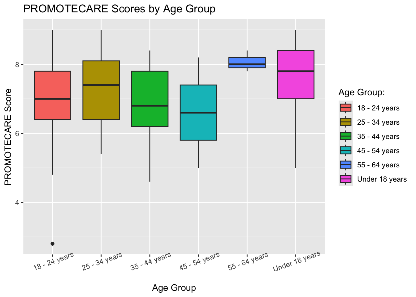
  • Age group does not appear to have a strong correlation with the PROMOTECARE score, although individuals in the 55-64 age group tend to have higher PROMOTECARE scores, which means they may have a stronger focus on creating positive outcomes for others.
Show the code
## PROMOTECARE score distributions across age group

age_procare <- ggplot(df, aes(x = demo6, y = PROMOTECARE, fill = demo6)) + 
  geom_boxplot() +
  labs(title ="PROMOTECARE Scores by Age Group", x ="Age Group", y ="PROMOTECARE Score")+
  guides(fill = guide_legend(title ="Age Group:"))+
  theme(axis.text.x = element_text(angle = 20))  


age_procare

3.3 Failing to Care Mindset by Racialized Identity

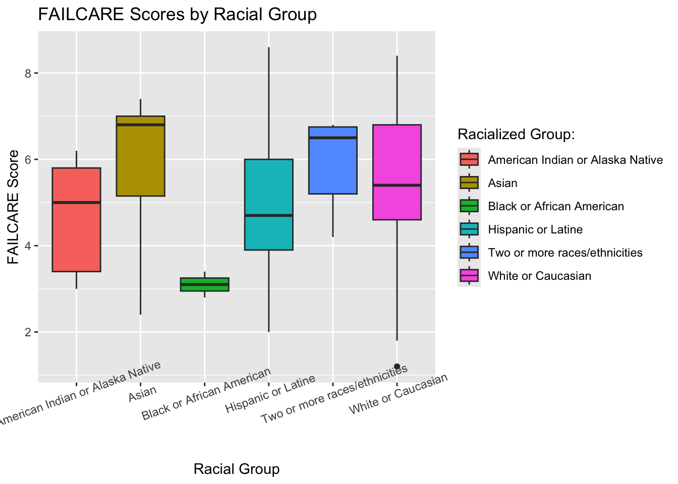
  • Racial group does not appear to have a strong correlation with the FAILCARE score, although people who identify as Asian tend to have higher FAILCARE scores, which means they have a greater worries about failing to create positive outcomes for others.
Show the code
## FAILCARE score distributions across racial group

racial_failcare <- ggplot(df, aes(x = demo2, y = FAILCARE, fill = demo2)) + 
  geom_boxplot() +
  labs(title ="FAILCARE Scores by Racial Group", x ="Racial Group", y ="FAILCARE Score")+
  guides(fill = guide_legend(title="Racialized Group:"))+
  theme(axis.text.x = element_text(angle = 20))  

racial_failcare

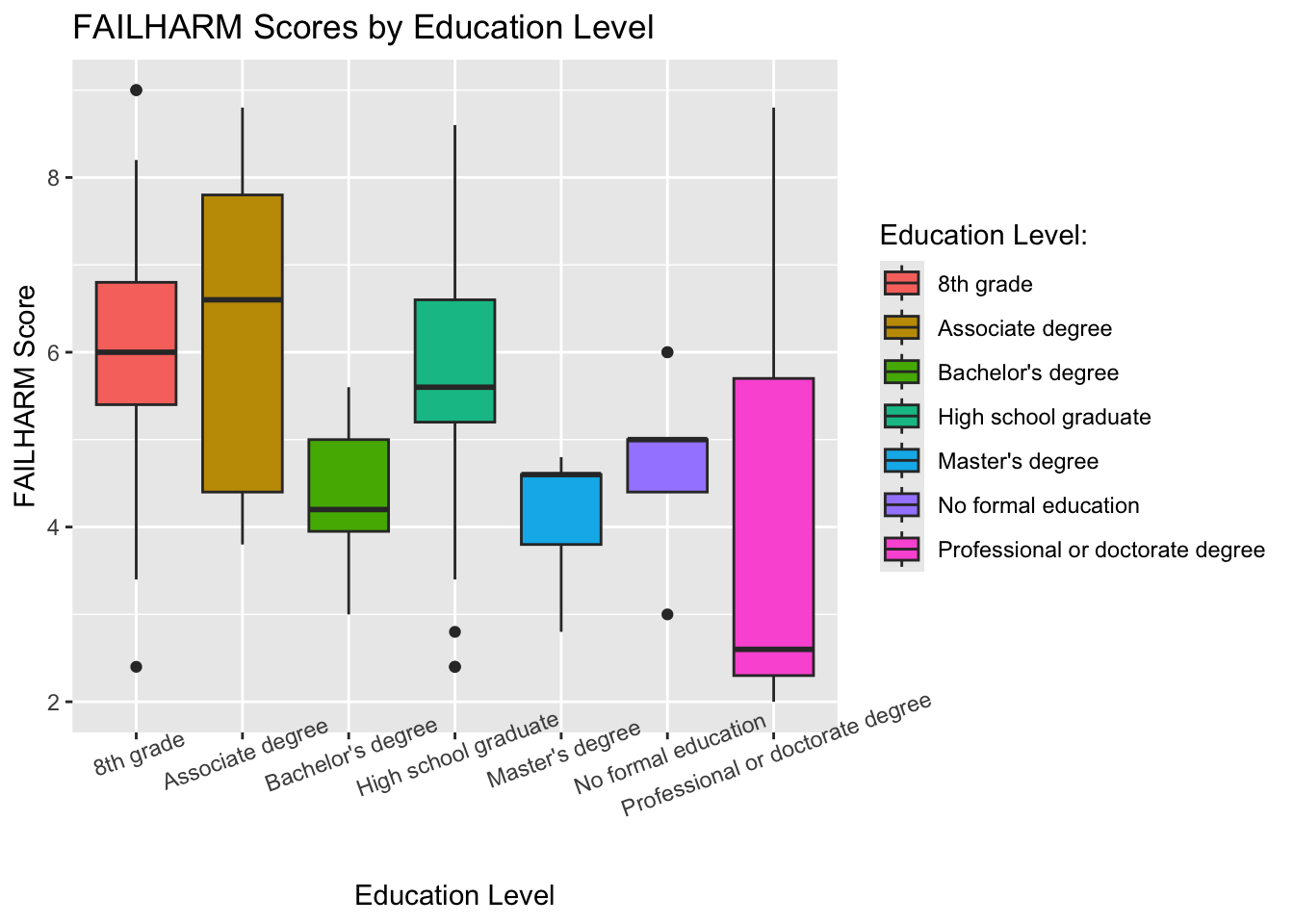
3.4 Failing to Prevent Harm Mindset by Educational Level

  • As education level increases, individuals endorse lower scores on failing to prevent harm mindset. Simply, this means more educated people have a less anxiety about failing to prevent negative outcomes.
Show the code
## FAILHARM score distributions across education level

education_preharm <- ggplot(df, aes(x = demo3, y = FAILHARM, fill = demo3)) + 
  geom_boxplot() +
  labs(title = "FAILHARM Scores by Education Level", x ="Education Level", y ="FAILHARM Score")+
  guides(fill = guide_legend(title ="Education Level:"))+
  theme(axis.text.x = element_text(angle = 20))

education_preharm

3.5 Paired Comparisons of PROMOTECARE vs. PREVENTHARM

Show the code
#df_zscore <- df_long %>%
  #mutate(zscore = scale(value))

#df_zscore
Show the code
## Compare PROMOTECARE vs. PREVENTHARM using violin plots

#procare <- ggplot(df_zscore, aes(x = variable, y = zscore)) +
  #geom_violin(aes(fill = variable),alpha = 0.6) +
  #geom_point(aes(group = participantID), size = 1.5, alpha = 0.4)+
  #geom_line(aes(group = participantID), color = "black", alpha = 0.3) +
  #scale_fill_manual(values=c("PROMOTECARE" = "#8297ce", "PREVENTHARM" = "#453a98")) +
  #labs(title="Comparison of PROMOTECARE vs. PREVENTHARM", x="Mindset", y="Z-score")

#procare  

4 Within-Person Analysis of Mindsets

4.1 Mindsets of Five Randomly Selected Participants

Show the code
## for reproducibility
set.seed(123)               
random_ids5 <- sample(unique(df$participantID), 5)

random_ids5
[1] 780121 559285 483997 589071 406263
Show the code
desired_order <- c("PROMOTECARE", "PREVENTHARM", "MAINTAIN", "RESPOND", "FLIP", "FAILCARE", "FAILHARM")

plot_mindsets <- function(person_id) {
  df_person <- df %>% 
    filter(participantID == person_id) %>% 
    select(PROMOTECARE, PREVENTHARM, FAILCARE, FAILHARM, MAINTAIN, FLIP, RESPOND) %>% 
    pivot_longer(cols = everything(), names_to = "variable", values_to = "value") %>%
    mutate(variable = factor(variable, levels = desired_order)) %>%
    mutate(zscore = scale(value))

  ggplot(df_person, aes(x = variable, y = zscore, group = 1)) +
    geom_point(size = 4, color = "#453a98") +
    geom_line(color = "#8297ce") +
    labs(
      title = paste("Comparison of All Mindset Scores for Participant", person_id),
      x = "Mindset", y = "Z-score"
    ) +
    theme_minimal() +
    theme(axis.text.x = element_text(angle = 20, hjust = 1))

}

plot_mindsets(random_ids5[1])

Show the code
plot_mindsets(random_ids5[2])

Show the code
plot_mindsets(random_ids5[3])

Show the code
plot_mindsets(random_ids5[4])

Show the code
plot_mindsets(random_ids5[5])

4.2 Combined Plot of Five Randomly Selected Participants

Show the code
#desired_order <- c("PROMOTECARE", "PREVENTHARM", "MAINTAIN", "RESPOND", "FLIP", "FAILCARE", "FAILHARM")

#df_plot <- df %>%
  #filter(participantID %in% random_ids5) %>%
  #select(participantID, PROMOTECARE, PREVENTHARM, FAILCARE, FAILHARM, MAINTAIN, FLIP, RESPOND) %>%
  #pivot_longer(
    #cols = -participantID,
    #names_to = "variable",
    #values_to = "value"
  #) %>%
  #group_by(participantID) %>%
  #mutate(variable = factor(variable, levels = desired_order)) %>%
  #mutate(zscore = scale(value)) %>%
  #ungroup()

#df_plot
Show the code
#ggplot(df_plot, aes(x = variable, y = zscore, color = participantID, group = participantID)) +
  #geom_point(size = 3) +
  #geom_line(size = 1) +
  #labs(
    #title = "Mindset Score Comparison (Z-Scores) for 5 Random Participants",
    #x = "Mindset Type",
    #y = "Z-score",
    #color = "Participant ID"
  #) +
  #theme_minimal() +
  #theme(axis.text.x = element_text(angle = 20, hjust = 1))

4.3 Mindsets of Ten Randomly Selected Participants

Show the code
## for reproducibility
set.seed(123)               
random_ids10 <- sample(unique(df$participantID), 10)

random_ids10
 [1] 780121 559285 483997 589071 406263 453579 391074 126294 570244 559835
Show the code
desired_order <- c("PROMOTECARE", "PREVENTHARM", "MAINTAIN", "RESPOND", "FLIP", "FAILCARE", "FAILHARM")

df_plot <- df %>%
  filter(participantID %in% random_ids10) %>%
  select(participantID, PROMOTECARE, PREVENTHARM, FAILCARE, FAILHARM, MAINTAIN, FLIP, RESPOND) %>%
  pivot_longer(
    cols = -participantID,
    names_to = "variable",
    values_to = "value"
  ) %>%
  group_by(participantID) %>%
  mutate(zscore = scale(value)) %>%
  mutate(variable = factor(variable, levels = desired_order)) %>%
  ungroup()

df_plot
# A tibble: 70 × 4
   participantID variable    value zscore[,1]
           <dbl> <fct>       <dbl>      <dbl>
 1        589071 PROMOTECARE   5       0.0725
 2        589071 PREVENTHARM   4.8    -0.0967
 3        589071 FAILCARE      5.4     0.411 
 4        589071 FAILHARM      2.6    -1.96  
 5        589071 MAINTAIN      4.6    -0.266 
 6        589071 FLIP          6.4     1.26  
 7        589071 RESPOND       5.6     0.580 
 8        780121 PROMOTECARE   8.6     1.01  
 9        780121 PREVENTHARM   3      -1.49  
10        780121 FAILCARE      7.8     0.650 
# ℹ 60 more rows
Show the code
ggplot(df_plot, aes(x = variable, y = zscore, color = participantID, group = participantID)) +
  geom_point(size = 3) +
  geom_line(size = 1) +
  labs(
    title = "Mindset Score Comparison (Z-Scores) for 10 Random Participants",
    x = "Mindset Type",
    y = "Z-score",
    color = "Participant ID"
  ) +
  theme_minimal() +
  theme(axis.text.x = element_text(angle = 20, hjust = 1))
Warning: Using `size` aesthetic for lines was deprecated in ggplot2 3.4.0.
ℹ Please use `linewidth` instead.
Warning: Removed 7 rows containing missing values or values outside the scale range
(`geom_point()`).
Warning: Removed 7 rows containing missing values or values outside the scale range
(`geom_line()`).

Show the code
library(patchwork)
Show the code
plots <- lapply(random_ids5, function(id) {
  plot_mindsets(id) + 
  theme(plot.title = element_blank()) # Remove individual plot titles
})

# Combine them with patchwork
combined_plot <- plots[[1]] + plots[[2]] + plots[[3]] + plots[[4]] + plots[[5]] +
  plot_layout(ncol = 2, nrow = 3) + 
  plot_annotation(title = "Mindset Score Comparison for 5 Random Participants")

combined_plot